· Matthias Quinn · 41 min read
Cluster Validity Indices
My master's thesis

Introducing a Python Package for Internal and External Cluster Validity Indices
Author: Matthias Quinn
Class: STA 696
Advisor: Dr. Richard Fan
Date Began: 28th February 2021
Semester: Fall 2021
Abstract
The following research examines various clustering methods and internal validity indices. Many clustering algorithms depend on various assumptions in order to identify subgroups, so there exists a need to objectively evaluate these algorithms, whether through complexity analyses or the proposed internal validity indices. The goal is to apply these indices to both artificial and real data in order to assess their fidelity. Currently, there exists no Python package to achieve this goal, but the proposed library offers indices to help the user choose the correct number of clusters in his/her data, regardless of the chosen clustering methodology.
1. Introduction
The goal of this project is to understand and compute a variety of indices that indicate the optimal number of clusters to use when performing a cluster analysis.
Cluster analysis refers to a finding unique subgroup/clusters in a dataset where the observations within each cluster are more related to each other in some way compared to observations in another, separate cluster. There are a plethora of clustering techniques and algorithms, each with a different way of solving the above general problem. In addition, there does not exist a single, optimal clustering solution for any clustering problem. This is also known as the “No Free Lunch” theorem from David Wolpert and William Macready, which states that “any two optimization algorthims are equivalent when their performance is averaged across all possible problems.” (Wolpert, Macready, 2005)
Since cluster analysis is inherently an unsupervised learning technique, the selection of the optimal number of clusters is subjective. Consider the following example that was made via Python:
from sklearn.datasets import make_blobs
import pandas as pd
from sklearn.cluster import KMeans
import matplotlib.pyplot as plt
import seaborn as sns

data, true_labels, _ = make_blobs(n_samples=500, n_features=2, centers = 4, random_state=1234, cluster_std=0.9)

points = pd.DataFrame(data, columns=['x', 'y'])

k4 = KMeans(n_clusters=4, random_state=1234).fit(points)
k5 = KMeans(n_clusters=5, random_state=1234).fit(points)
k6 = KMeans(n_clusters=6, random_state=1234).fit(points)

fig = plt.figure(figsize=(12, 12))
ax1 = fig.add_subplot(221)
ax2 = fig.add_subplot(222)
ax3 = fig.add_subplot(223)
ax4 = fig.add_subplot(224)

ax1.scatter(points['x'], points['y'], color="black")
ax1.axes.get_xaxis().set_visible(False)
ax1.axes.get_yaxis().set_visible(False)
ax2.scatter(points['x'], points['y'], c=k4.labels_.astype(float))
ax2.axes.get_xaxis().set_visible(False)
ax2.axes.get_yaxis().set_visible(False)
ax3.scatter(points['x'], points['y'], c=k5.labels_.astype(float))
ax3.axes.get_xaxis().set_visible(False)
ax3.axes.get_yaxis().set_visible(False)
ax4.scatter(points['x'], points['y'], c=k6.labels_.astype(float))
ax4.axes.get_xaxis().set_visible(False)
ax4.axes.get_yaxis().set_visible(False)

ax1.title.set_text('Original Data')
ax2.title.set_text('K=4 Clusters')
ax3.title.set_text('K=5 Clusters')
ax4.title.set_text('K=6 Clusters')

plt.show()
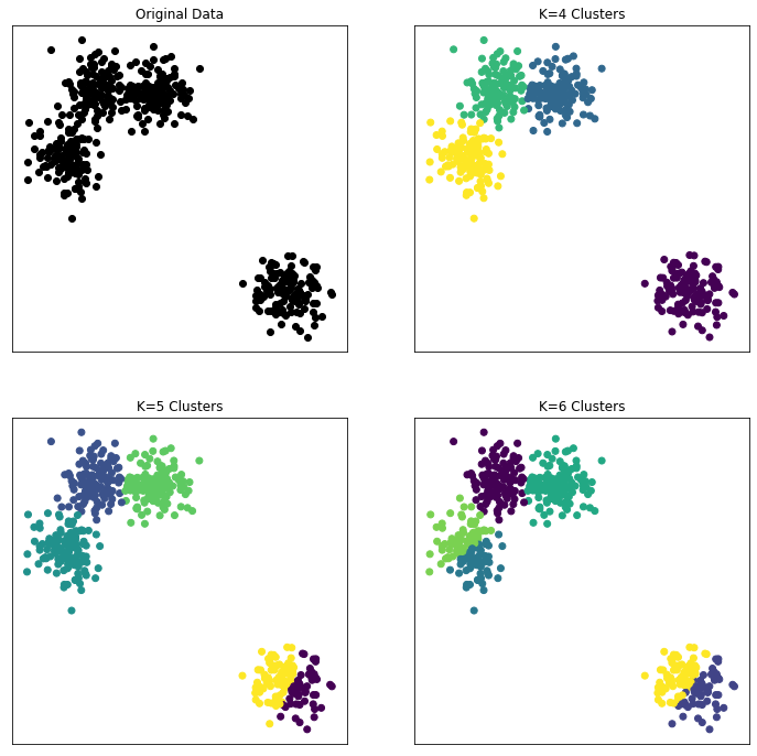
The figure above helps to illustrate that the definition of a cluster is imprecise and that the best definition depends on the nature of the data and the user’s desired results.
2. Methods
2.1 Language
Python was chosen as the language of choice due to the author’s familiarity with the various libraries made available in Python, including the NumPy and Sci-kit Learn modules. R was heavily used to double-check many of the algorithms and indices, relying mostly on the NbClust library (Charrad, 2014).
2.2 Related Work
A variety of measures aiming to validate the results of a cluster analysis have been defined over the years and this project focuses on relative criteria, which consists of the evaluation of a clustering algorithm by comparing it with the same algorithm but varies in the input parameters.
The inspiration for this project came on the heels of a separate project where a cluster analysis was used, but choosing the number of clusters appropriate for the final conclusion was unclear, both numerically and graphically. R has great support for cluster analysis and choosing the number of clusters; in particular, the NbClust package provides extensive support for both tasks and is the main inspiration for this project. The R package came out in October 2014 and contains a variety of indices that help aid the user in choosing the appropriate number of clusters, given one of two clustering methods; namely, K-Means and agglomerative clustering.
However, when looking to validate results in another language, there was an apalling lack of libraries available for accomplishing the task. Python lacks, and still does as of writing, a comprehensive package for choosing an appropriate number of clusters. Python’s Sci-kit Learn library does have support for a plethora of clustering algorithms, including the ones used in this project, as well as a few others. However, it only supports three clustering indices.
The three clustering indices covered by Python’s Sci-kit Learn library are the silhouette coefficient, the Davies-Bouldin index, and the Calinski-Harabasz index. The proposed library, as well as NbClust, support all three of the indices in addition to many more.
3. Clustering Algorithms
It is worth mentioning that the algorithms discussed below are not an exhaustive list of potential clustering methods and the proposed Python package supports any method that produces predictive labels. Also, R’s NbClust package only supports two clustering algorithms at the moment; namely, K-Means and Hierarchical clustering.
3.1 K-Means
The K-Means algorithm is a centroid-based clustering technique and is one of the most popular clustering algorithms, so it had to be covered. A slight alternative to the algorithm, K-medians, uses the median instead of the mean, but will not be covered in this project. The algorithm attempts to minimize the within-cluster variances, which will be formalized next.
3.1.1 The K-Means Algorithm
Given a set of n observations each consisting of d dimensions, and wanting to partition those observations into k clusters, the goal is to minimize the within-cluster sum of squares (WSS). Formally, the K-Means algorithm is as follows:
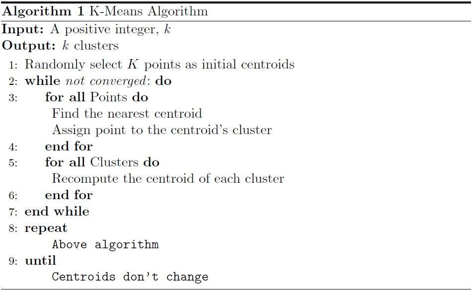
Initially, points are assigned to the initial centroids, which in this case is the mean. After the points are assigned to the centroid, the centroid is then updated until no more changes occur and the algorithm converges. There is no guarantee, however, that the algorithm will converge. The objective is to minimize the pairwise squared deviations of points in the same cluster:
The within cluster sum of squares, or what the Sci-kit Learn package calls inertia, is a measure of how internally coherent separate clusters are. The optimal value is 0 while lower values indicate more separated clusters. Sci-kit Learn uses Lloyd’s algorithm which follows the steps in the algorithm presented above and uses the squared Euclidean distance.
3.1.2 Time and Space Complexity
K-Means only needs to store the data points and each centroid. Specifically, the storage requirements for the algorithm is , where m is the number of data points, n is the number of variables, and K is the pre-specified number of clusters. K-Means runs in linear time, in particular, , where is the number of iterations until convergence. As long as the number of clusters remains significantly below the number of variables, the K-Means algorithm should run in linear time.
3.2 Agglomerative Hierarchical Clustering
Another commonly-used approach for clustering is that of hierarchical clustering, of which, there are two approaches; namely, Agglomerative, and Divisive.
Agglomerative: Start with clusters and keep going until you have cluster.
Divisive: Start with cluster and decompose until you have clusters.
This section will focus solely on the Agglomerative variant.
3.2.1 Agglomerative Hierarchical Clustering Algorithm
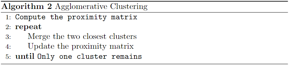
The key operation of the Agglomerative Clustering algorithm is the calculation of the proximity between two clusters, where the definition of cluster proximity differentiates the various agglomerative flavors.
Ward’s method assumes that a cluster is represented by its centroid, but it measures the proximity between two clusters in terms of the increase in the SSE that results from merging the two clusters. Ward’s method attempts to minimize the sum of the squared distances of points from their cluster centroids. The initial cluster distances in Ward’ minimum variance method are defined to be the squared Euclidean distance between points:
3.2.2 Time and Space Complexity
Ward’s method requires the storage of where is the number of datapoints and the storage required to keep track of the clusters is proportional to the number of clusters, which is , excluding singleton clusters. Thus, the total space complexity of Ward’s method is .
Next, in terms of the time required to run the algorithm, a good place to start is the computation of the proximity matrix. time is required to compute the proximity matrix. Afterwards there are iterations involving steps and because there are clusters at the start and two clusters are merged after each iteration. In addition, because the algorithm exhaustively scans the proximity matrix for the lowest distances, the run time is .
Obviously, because of the rather large space and time complexity of the Agglomerative Clustering algorithm, it should not be used for large datasets. In addition, the Agglomerative Clustering algorithm tends to make good local decisions about which two clusters to combine since they can use information about the pairwise similarity of all of the data points. However, once a decision is made to merge two clusters, the merge is final and it cannot be undone.
3.3 DBSCAN
Density-based clustering locates regions of high density that are separated from one another by regions of low density. A cluster is considered to be a set of core samples and a set of non-core samples that are close to a core sample. In this approach, known as the center-based approach, the density for a particular point is estimated by counting the number of points within a specified radius, which is controlled by the Epsilon parameters.
There are three types of data points of consideration in the DBSCAN algorithm, namely:
Core points: The points are inside the interior of a density-based cluster. A point is a core point if the number of points within a given neighborhood around the point exceeds a certain threshold, minsamples, as defined by _Sci-kit Learn.
Border points: A point that is not a core point, but rather falls within the neighborhood of a core point, which can fall within the neighborhood of several core points.
Noise points: Any points that is neither a core point nor a border point.
An example of the three points described above are shown below:
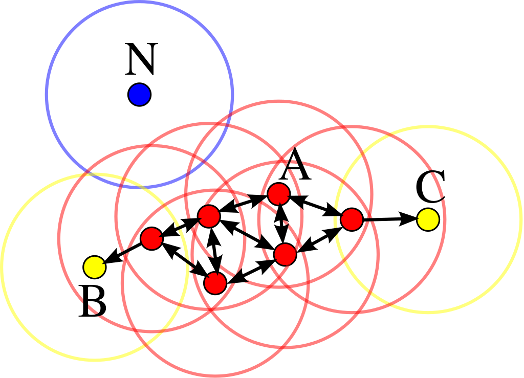
Fig. 4 - Demonstration of Core, Border, and Noise points present during the usage of the DBSCAN algorithm
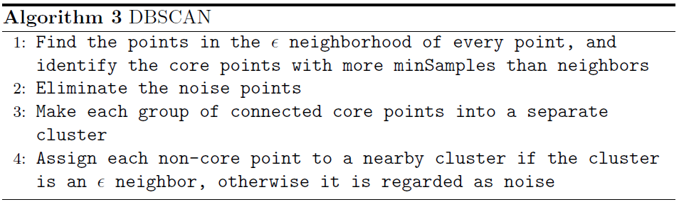
3.3.1 The DBSCAN algorithm
Informally, any two core points that are close enough, within a distance of the Epsilon parameter, are put into the same cluster. Additionally, any border point that is close enough to a core point is put in the same cluster as the core point. Finally, noise points are discarded. More formally:
3.3.2 Time and Space Complexity
In the worst case, the time complexity of the DBSCAN algorithm is , where is the number of data points, since DBSCAN visits each point of the data set. In Sci-kit Learn, the DBSCAN implementation uses two tree data structures, namely, ball trees and kd-trees, to determine the neighborhood of points. In particular, the kd-tree allows for the efficient retrieval of all points within a given distance of a specified points, meaning the time complexity for the DBSCAN algorithm can be as low as
The implementation of the DBSCAN algorithm in Sci-kit Learn consumes floats, but this can be reduced to since it is only necessary to store the cluster label and what type of point each datum belongs to.
4. Internal Cluster Validity Indices
Users often have to select the best number of clusters in a data set without some indication of what the correct number of clusters should be. In addition, different clustering algorithms can lead to different clusters of the data. In addition, using different parameters for the same algorithm can also lead to different clustering results.
Since the need for effective evaluation standards has been described, this section will focus on a variety of indices that can be used to aid the user in selecting an appropriate amount of clusters.
4.0 Notation:
This section contains information on notations used throughout the rest of the paper.
Let us denote the following:
= total number of observations in a dataset
= the total number of numeric variables used to cluster the data
= the total number of clusters
= the data matrix of shape
= A submatrix of made up of the rows of where some partition, , contains any point belonging to cluster
= the number of observations belonging to cluster
4.1 Ball-Hall Index
This index is based on the average distance of the items to their respective cluster centroids. It is just the within-group sum of distances and is computed as:
where is the within-group dispersion matrix for the data clustered into clusters. This index requires the computation of centroids and within-group distances, which itself is . Thus, Ball-Hall is where is the number of variables in the data set to be clustered.
The maximum difference in the Ball-Hall indices between different clusters is considered to be the optimal number of clusters.
4.2 The Beale Index
Beale, 1969 introduced the idea of using an F-ratio to test the hypothesis of the existence of versus clusters in the data (). The optimal number of clusters is obtained by comparing with an distribution, where the null hypothesis would be rejected for significantly large values of the F-statistic. In the proposed Python package, the user can control the level used to compute the critical value, and the default value is .
Mathematically, the calculation of the Beale index is as follows:
where and is the number of variables.
4.3 The C Index
The C index was reviewed by Hubert and Levin, 1976 and is calculated below:
where
= the sum of the smallest distances between all the pairs of points in the entire data set;
= the sum of the largest distances between all the pairs of points in the entire data set.
=
The optimal number of clusters is indicated by the minimum value of the C index. Finally, the C-index has a time complexity of , mostly due to the computational cost of sorting the pairwise distances, which can be slow with a large number of observations.
4.4 The Calinski-Harabasz Index
The Calinski-Harabasz index Calinski, Harabasz, 1974, also known as the Variance Ratio Criterion, is a measure of how similar an object is to its own cluster compared to other clusters. From Sci-kit Learn’s website, the score is defined as the ratio between the within-cluster dispersion and between-cluster dispersion. More formally put:
where:
and:
and: ,
where is the attribute of the data object and is the attribute of the centroid of the cluster.
The maximum value of the CH score, given a range of clusters, is considered to be the best number of clusters. The Calinski-Harabasz index also has complexity.
4.5 Cubic Clustering Criterion
The CCC by Sarle, 1983 is obtained by comparing the observed to the approximate expected using an approximate variance-stabilizing transformation. CCC values greater than 0 mean that the obtained is greater than would be expected if sampling from a uniform distribution. According to the SAS Institute, the best way to use the CCC is to plot its values against the number of clusters. The CCC is used to compare the you obtain for a given set of clusters with the you would get by clustering a uniformly/normally distributed set of points in dimensional space. In addition, the optimal number of clusters is indicated by the maximum CCC value. Mathematically, the CCC can be computed as follows:
where,
and,
and,
and,
and,
and,
is the largest integer less than such that is not less than one.
Finally, the reason for the odd ending to the expected r-squared formula was derived empirically to stabilize the variance across different combinations of observations, variables, and clusters.
4.6 D Index
The D Index from Lebart et al., 2000 is based on clustering gain on intra-cluster inertia, which measures the degree of homogeneity between the data associated with a cluster. It calculates their distances compared to the cluster centroid.
Mathematically, intra-cluster inertia is defined as:
The clustering gain on the intra-cluster inertia, given two partitions, composed of clusters and composed of clusters, is defined as:
The clustering gain above should be minimized. In addition, the optimal suggested number of clusters corresponds to a significant decrease of the first different of clustering gain, compared to the number of clusters. This “significant decrease” can be identified by examining the second differences of clustering gain.
4.7 Davies-Bouldin Index
The Davies-Bouldin Index is a function of the sum ratio of within-cluster scatter to between-cluster separation. A lower value indicates a better clustering solution, i.e. better separation between the clusters.
Mathematically, the index is defined as the average similarity between each cluster and its most similar one, where the similarity is defined as a measure that is nonnegative and symmetric, like so:
Then the Davies-Bouldin index is defined as:
Finally, in terms of computational complexity, the Davies-Bouldin index runs in time.
4.8 Duda Index
The Duda index, Duda and Hart, 1973 is the ratio between the sum of squared errors within clusters when the data are partitioned into two clusters, and the squared errors when only one cluster is present.
Mathematically, this can be represented as:
The optimal number of suggested clusters is the smallest such that:
where 3.20 is a Z-score tested by Milligan and Cooper, 1985
4.9 Dunn Index
The Dunn index (Dunn, 1974) is the ratio between the minimal intercluster distance to the maximal intracluster distance. If the data set contains well-separated clusters, the diameter of the clusters is expected to be small and the distance between the clusters should be large. Thus, the suggested optimal number of clusters corresponds to the maximum value of the Dunn index.
Mathematically:
where:
and,
and is known as the diameter of a cluster, or the largest distance separating two distinct points in a particular cluster.
In terms of computational complexity, the Dunn index runs in time.
4.10 Frey Index
The Frey index,proposed by Frey and Van Groenewoud, 1972, is the ratio of the difference scores from two successive levels in a hierarchy. This means that the index should only be used on hierarchical clustering method. The numerator represents the difference between the mean between-cluster distances while the denominator represents the difference between the mean within-cluster distances, each from the two levels.
Mathematically, the Frey index can be written as:
where the mean between-cluster distance is:
and the mean within-cluster distance is:
The best clustering solution occurs when the ratio falls below 1.0, and the cluster level before that point is taken as the optimal partition. In addition, if the ratio never falls below 1.0, a one cluster solution is usually best.
4.11 Gamma Index
The Gamma Index compares all within-cluster dissimilarities and all between-cluster dissimilarities. A comparison is concordant/discordant if a within-cluster dissimilarity is less/greater than a between cluster dissimilarity. Ties are disregarded. Also, the maximum value of the index indicates the optimal suggested number of clusters.
Mathematically, the Gamma Index is defined as:
where,
is the number of concordant comparisons
and,
is the number of discordant comparisons
Furthermore, the definition of concordant and discordant pairs is defined mathematically below:
and,
where,
if the corresponding inequality is satisfied and otherwise.
In terms of computational complexity, this index requires the computation of all pairwise distances between objects, which itself is . In addition, computing and requires time, so the total computational cost of the Gamma index is . This index should almost never be used for large data sets as it is very resource heavy. The performance of this particular index, along with the G+ and Tau indices, will be discussed in the performance section later on.
4.12 G-Plus Index
The G+ index is another metric based on the relationships between just the discordant pairs of objects, . It is simply the proportion of discordant pairs with respect to the maximum number of possible comparisons. The optimal number of clusters in the data is given by the minimum value of the index.
Mathematically, the index can be computed as:
The computational run time of the G+ index is also and as such should not be used for larger data sets.
4.13 Hartigan Index
The Hartigan index is based on the Euclidean within-cluster sums of squares. The optimal number of clusters is given by the maximum difference between successive clustering solutions.
Mathematically, it can be expressed as:
where is the within-cluster dispersion matrix for the data clustered into clusters
The computational run time of the Hartigan index is and is discussed in further detail ahead.
4.14 Log SS Ratio Index
This index, from J. A. Hartigan. Clustering algorithms. New York: Wiley, 1975. considers the within () and between () cluster sums of squares. It should be noted that the log used is base , not .
The time complexity of this index is, at worst, and at best when . Thus, this index is ideal for data with naturally large clusters.
4.15 Marriot Index
The Marriot Index Marriot, 1971 is based on the determinant of the within-group covariance matrix.
Mathematically, it is computed as:
The suggested optimal number of clusters is based on the maximum difference between successive levels of the Marriot index. The overall computational complexity of the Marriot index is , making it suitable for large datasets with a medium number of dimensions.
4.16 McClain Index
The McClain and Rao index McClain and Rao, 1975 is the ratio of the average within cluster distance - divided by the number of within cluster distances - and the average value between cluster distances - divided by the number of cluster distances.
Mathematically, it is formed by:
The optimal suggested number of clusters corresponds to the minimum value of the index. Finally, in terms of computational complexity, the McClain Rao index runs in time.
4.17 Point-Biserial Index
The Point Biserial index is the point-biserial correlation between the dissimilarity matrix and a corresponding matrix consisting of either 0’s or 1’s. A value of is assigned if the two corresponding points are clustered together by the algorithm and otherwise.
Mathematically, the index is defined as:
where,
and,
and,
is the standard deviation over all of the distances
and,
= The number of data points in each cluster, so an array of length
= = Total number of pairs of distinct points in the data set.
= = The number of paris of points belonging to clusters and .
= = The number of pairs of points belonging to clusters and where and are not the same cluster.
In terms of computational complexity, the Point-Biserial index takes time to be computed.
4.18 Pseudo T2 Index
The Pseudo index from Duda and Hart, 1973 can only be applied to hierarchical clustering methods, but is included for all clustering methods in the proposed Python package. This is because the user should understand that the metric should only be used for that specific method.
Mathematically, the index is computed as:
The suggested optimal number of clusters is based on the smallest such that:
4.19 Ratkowsky-Lance Index
The Ratkowsky and Lance, 1978 index is based on the average of the ratio between the between-group sum of squares and the total sum of squares for each variable.
Mathematically, it is computed as:
where,
and,
and,
The optimal number of clusters is suggested by the maximum value of the index. Finally, the index runs in time.
4.20 Ray-Turi Index
This index, proposed by Ray and Turi in 1999, came off of the heels of image segmentation, which separates parts of images into differing components. The index is simply the ratio between the intra-cluster distance and the inter-cluster distance.
Mathematically, it can be written as:
where:
and,
and is the centroid of cluster
Since the goal is to minimize the intra-cluster distance - the numerator - the optimal cluster partitioning corresponds to the minimum value of the Ray-Turi index.
4.21 R Squared Index
While not included as part of the NbClust standard library, the index is inherently necessary to compute, since it is relied upon by the cubic clustering criterion, as mentioned above. The maximum difference between successive clustering levels is regarded as the best partition. The mathematical formulation is as follows:
where:
and,
is the total sum of squares and cross-products matrix of shape .
4.22 Rubin Index
The Rubin Index, proposed by Friedman and Rubin in 1967, is based on the ratio of the determinants of the data covariance matrix and within-group covariance matrix.
Mathematically, it can be formed like so:
The optimal clustering solution is given by the minimum value of the second differences between clustering levels. In terms of computational complexity, the Rubin index runs in time.
4.23 Scott-Symons Index
The Scott-Symons index, Scott and Symons, 1971, uses information from the determinants of the data covariance matrix and the within-group covariance matrix, similar to the Rubin index.
Mathematically, it can be written as:
where:
and,
The optimal suggested number of clusters is given by the maximum value of the index. Finally, the index runs in time.
4.24 SD Index
The SD validity index is based on the concepts of average scattering for clusters and total separation between clusters.
Mathematically, it is computed as:
The scattering term, or the average compactness of clusters, is computed as:
where:
and is the maximum distance between cluster centers and is the minimum distance between cluster centers. In addition, is the vector of variances for each variable in the data set and is the variance vector for each cluster, .
It should be noted that is a weighting factor equal to Dis() where is the maximum number of clusters. The optimal suggested number of clusters is indicated by the minimum value of the SD index.
4.25 SDbw Index
The SDbw index is based on the compactness and separation between clusters.
Mathematically, it can be computed as:
where:
and,
The term is calculated in the same way as above. The new term - - is the inter-cluster density, which is the average density in the region among clusters in relation to the density of the clusters.
The optimal number of clusters is the partition that minimizes the SDbw index.
4.26 Silhouette Score
Introduced by Rousseeuw in 1987, the Silhouette Coefficient is composed of two scores:
a: The mean distance between a sample and all other points in the same class
b: The mean distance between a sample and all other points in the next nearest cluster
Mathematically, this can be written as:
Additionally, the Silhouette Score for a set of sample is just the mean Silhouette Coefficient for each sample, like so:
where:
and,
and,
The optimal number of clusters is indicated by the maximum value of the index. Scores around indicate overlapping clusters. Finally, the index can be calculated in time.
4.27 Tau Index
The Tau index is based on the correlation between the matrix that stores all of the distances between pairs of observations and a matrix that represents whether a given pair of observations belongs to the same cluster or not. It can be written in terms of concordant and discordant pairs of observations, just like the Gamma and G+ indices.
Mathematically, it can be written as:
where is the total number of distances and is the number of comparisons between two pairs of observations.
The optimal suggested clustering solution is given by the maximum value of this index. In terms of computational complexity, the Tau index runs in the same time as the Gamma index; namely, making it suitable for small datasets.
4.28 Trace-Cov-W Index
The Trace(Cov(W)) index involves using the pooled covariance matrix instead of the within-group covariance matrix.
Mathematically, it can be written as:
where:
and,
and,
The optimal suggested number of clusters is indicated by the maximal difference in index scores. Finally, in terms of computational efficiency, the index can be calculated in time, making it ideal for larger data sets.
4.29 Trace-W Index
The Trace(W) index is a simple, difference-like criterion and is one of the most popular choices when selecting the appropriate number of clusters.
Mathematically, it can be calculated as:
where is the within-group covariance matrix.
The optimal suggested number of clusters corresponds to the maximum value of the second differences of the index. Finally, in terms of computational complexity, the index runs in time, making it ideal for large data sets.
4.30 Wemmert-Gancarski Index
The Wemmert-Gancarski index, is simply the weighted mean of the quotient of distances between a set of points and the barycenter of the cluster those points belong to.
Mathematically, it can be calculated as:
where:
and,
is the cardinality / number of points in a particular cluster
and:
4.31 Xie-Beni Index
The Xie-Beni index is an index primarily applied to fuzzy clustering solutions. It is defined as the quotient between the mean quadratic error and the minimum of the minimal squared distances between the points in the clusters.
Mathematically, the index can be calculated as:
where:
and is the distance between the cluster centroids.
The optimal suggested number of clusters corresponds to the minimum value of the index.
5. Library Performance
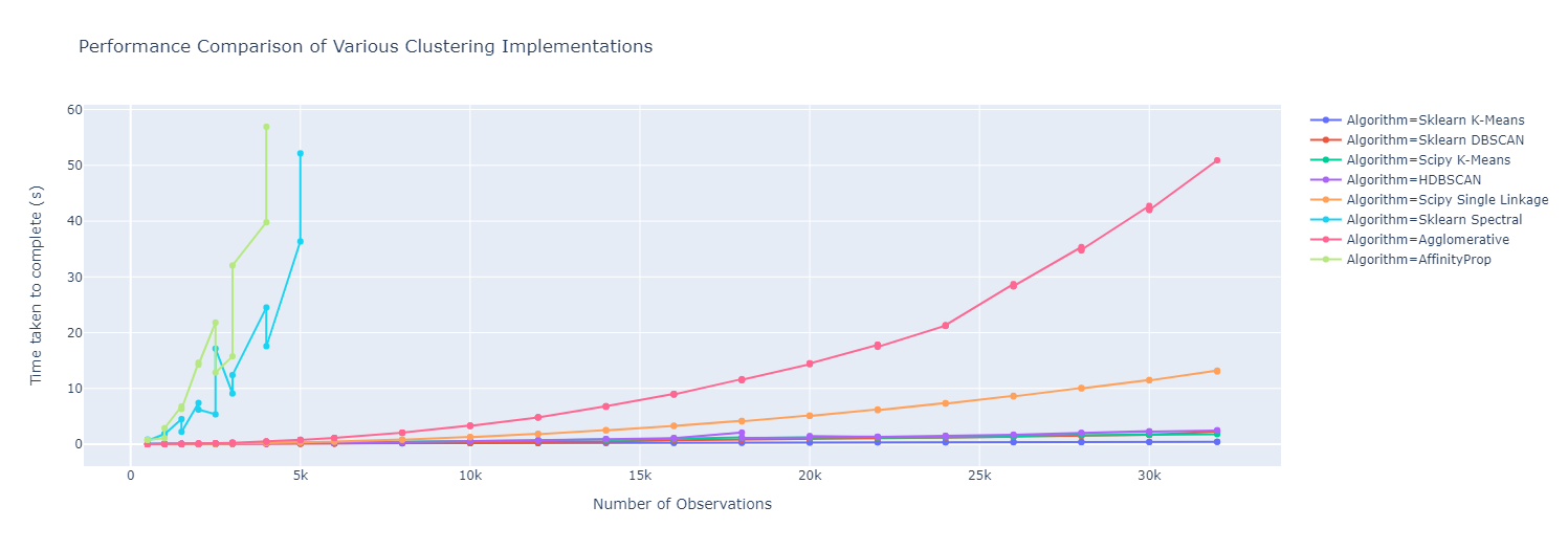
5.1 Testing Different Clustering Implementations
!pip install --upgrade pip
!pip install hdbscan
Import the necessary libraries
import hdbscan
import sklearn.cluster
import scipy.cluster
import sklearn.datasets
import numpy as np
import pandas as pd
import time
import matplotlib.pyplot as plt
import seaborn as sns
import plotly.express as px
import plotly.graph_objects as go
%matplotlib inline
sns.set_context('poster')
sns.set_palette('Paired', 10)
sns.set_color_codes()
Creating sample dataframes to cluster via NumPy.
dataset_sizes = np.hstack([np.arange(1, 6) * 500, np.arange(3,7) * 1000, np.arange(4,17) * 2000])
Benchmarking our data and clustering algorithms:
k_means = sklearn.cluster.KMeans(10)
k_means_data = benchmark_algorithm(dataset_sizes, k_means.fit, (), {})

dbscan = sklearn.cluster.DBSCAN(eps=1.25)
dbscan_data = benchmark_algorithm(dataset_sizes, dbscan.fit, (), {})

scipy_k_means_data = benchmark_algorithm(dataset_sizes,
                                         scipy.cluster.vq.kmeans, (10,), {})

scipy_single_data = benchmark_algorithm(dataset_sizes,
                                        scipy.cluster.hierarchy.single, (), {})

hdbscan_ = hdbscan.HDBSCAN()
hdbscan_data = benchmark_algorithm(dataset_sizes, hdbscan_.fit, (), {})

agglomerative = sklearn.cluster.AgglomerativeClustering(10)
agg_data = benchmark_algorithm(dataset_sizes,
                               agglomerative.fit, (), {})

spectral = sklearn.cluster.SpectralClustering(10)
spectral_data = benchmark_algorithm(dataset_sizes,
                                    spectral.fit, (), {})

affinity_prop = sklearn.cluster.AffinityPropagation()
ap_data = benchmark_algorithm(dataset_sizes,
                              affinity_prop.fit, (), {})
Plotting the results:
5.2 Indices Performance
This part will pertain to demonstrating the efficiency of the various clustering metrics offered by the proposed library. In addition, it will detail the various methods used to improve upon the efficiency of previous implementations, if they exist.
5.2.1 Ball-Hall Index:
The Ball-Hall Index is a relatively simple index that is essentially the mean dispersion of all points, relative to the cluster they belong to. As such, the index can be computed in time, making it ideal for larger datasets since it only requires computing the centroids of each cluster and the distances of each point within each cluster.
The author’s first attempt at implementing the index was unsuccessful, mostly due to a lack of understanding of the index. As a result, the initial run will not be used as a comparison and instead, only the NbClust version and the author’s new version will be compared.
Starting with the NbClust algorithm first, for a dataset with shape and , the mean time to compute the index was 0.01027 seconds for trial runs. In addition, the mean amount of resources used to compute the index was around MiB. In contrast, the new, working implementation included in the proposed library had a mean run tim of 0.00257 seconds, using the same circumstances as the first experiment. In addition, the mean amount of memory used was around MiB, used to store the new, split dataframes from the for-loop.
All together, the new, proposed implementation offers about a speedup and uses around of the memory. Reasons for these improvements come mostly from NbClust’s use of the sweep function to compute the mean differences, as well as the multiple uses of the split function, which splits a dataframe into chunks.
5.2.2 Index:
The author does not believe the NbClust library calculates the index correctly. For instance, while the source code for the index correctly calculates the number of within-cluster distances, , it does not correctly compute the sum of the largest/smallest pairwise distances, and respectively. In addition, it does not utilize a sorting/partitioning method of any kind, which is necessary for finding the largest/smallest pairwise distances.
To alleviate this problem, I rewrote the index to account for all parts of the original equation, from Hubert and Levin, 1976.
In terms of performance, the NbClust implementation will not be considered, for reasons listed above. It should be noted that a previous implementation of the index was made available in the Python language by John Vorsten in 2020, around the same time that I was working on this very project.
As stated previously, the index can be computed in time, which can be prohibitive if the number of variables used in the clustering is large. For reference, when , the number of pairwise distances is ; for observations, the number of pairwise distances is . Using the above example, the mean time to compute the index via John’s implementation was 27.5 seconds, compared to the proposed library’s mean run-time of 8.31 seconds.
The largest bottleneck in computing this index is calculating and , because it requires - at minimum - time to locate the smallest/largest pairwise distances. The main difference between the proposed library’s implementation and John’s is the calculation of and . In particular, John’s approach uses Numpy’s sort function, which by itself run’s in time, because the underlying algorithm used is a quicksort. However, the new library utilizes Numpy’s partition function, which runs in time, via the introselect algorithm, and does not require sorting the largest/smallest arrays.
5.2.3 Dunn Index:
The Dunn index requires the computation of the entire pairwise distance matrix, just like the index above, and has a time complexity of . This becomes a problem as grows large, but can be dealt with by precomputing the distance matrix and storing it in memory to query when needed. This reduces the time complexity of the algorithm to just , where is the number of clusters under consideration.
In a more practical setting, for a dataset with dimensions and , the mean time to compute the Dunn index, without precomputing the pairwise distances, is seconds via the proposed Python library. In contrast, the mean time to compute the same index with the same controls in place is seconds via the NbClust library. However, when utilizing a pre-computed distance matrix, the times fall to seconds and seconds for the proposed library and NbClust library, respectively.
The reasoning behind the solution lies behind the fact that in order find the maximum diameter / minimum intercluster distance, it requires a nested for-loop, which is used to go through each of the labels. Indexing an array takes time, so that lookup is dominated by the outer loops in the expression.
5.2.4 Hartigan Index:
Hartigan is credited with two internal clustering indices, the Hartigan Index and the Log Between/Within SS Index. This section will focus on the Hartigan index mentioned in the NbClust library. It was previously mentioned that the index runs in time, which can be quite fast when the number of requested clusters is small and the number of observations is also relatively small.
In the original implementation from the NbClust library, using the same setup as above, the index had a mean run-time of seconds and used about MiB of memory to compute. In contrast, the proposed library had a mean run-time of seconds and used about MiB of memory. For easier reference, the proposed library offers around a performance gain while utilizing about less memory.
It should be noted that both implementations perform fairly well on most datasets, so long as the dimensions of the dataset are of medium-size or lower.
5.2.5 Point-biserial Index:
As mentioned earlier, the point-biserial index, referenced as the PB index from here on, runs in time, where is the number of variables being clustered. However, an original implementation of the algorithm to compute the PB index runs in time, on average. For smaller inputs, this difference in run-time may be negligible; however, for larger datasets, the speed-up is quite dramatic. Using posterior analysis, the proposed library offers a speed-up in run-time up to 2600% ().
The main bottlenecks to the original implementation were, in decreasing order of execution time: the double for-loop to compute the distances and the design arrays ( = 112.5 seconds), converting the design array to a factor ( = 84 seconds), and garbage collection ( = 43.5 seconds).
A few methods were employed to improve upon the efficiency of the R implementation. Firstly, the design vector was discarded in favor of computing the number of points within/between the given clusters (), which both run in time instead of time, since the most tedious computation is counting the number of labels in each cluster. In addition, the biserial function used in NbClust’s version uses a separate code block to compute the biserial correlation between the design matrix and the distances, even though both libraries employ the following equality:
5.2.6 Index:
The Index has the usual interpretation of the amount of variation explained by the clustering solution. It should also be noted that the index is not the best method of criterion if your clustering solution is irregularly shaped or highly elongated.
Regarding the time complexity, the original implementation of the algorithm ran in time. This is because the algorithm has to, for each cluster and for each variable : compute the euclidean distance between the cluster center and the observation , write the product to an array, and then sum the result. The reasoning for the in the computation is because the euclidean distance requires time to be computed. For datasets with lots of observations and many variables to cluster, this time can be infeasible to work with.
The new algorithm offers a speedup in compute time, since it does not rely on a double for-loop or the computation of euclidean distances. Rather, it takes the raw data matrix and labels and computes a series of matrix multiplications.
5.2.7 Wemmert-Gancarski Index:
The Wemmert-Gancarski Index was an interesting metric since there was not a lot of literature regarding this index. For reference, the main source for the mathematical formulation of this index was the clusterCrit library vignette.
Initially, the index seemed a bit daunting since a plethora of methods were tried but none of them worked out. Instead, it required a pivot in thinking about how to structure and implement; rather than thinking about building the index in terms of what the output of each step should be, a shape-first approach was taken. More specifically, there were 5 steps to successfully implement the index using the approach of output shapes rather than just the output itself. A diagram of the author’s approach is shown below for easier reference:
WG Index:
Regarding the computational cost of computing the WG index, the modified OpenEnsembles version of the WG index had a mean run time of seconds; this is in stark contrast to the author’s proposed implementation that runs in seconds. The proposal is not only more than times faster than the previous implementation, but it also uses less memory as well (not a significant difference). Using the same setup as the other indices previously described, the mean amount of memory used per run for the new algorithm was around MiB, compared to the original implementation’s MiB memory usage; or less memory.
It should be noted that there were two resource-demanding tasks in the proposed implementation: namely, finding a quotient and finding the distances from each point to its centroid. Finding the quotient between the distance from a point to its barycenter and the minimum distance from a point and all of the other barycenters took, on average, only seconds. Finding the distances from all of the points to their centroids resulted in a mean run time of about seconds, using the same setup as above. Finally, the same tasks that were bottlenecks for the new version were also present in the old implementation, but the key difference lies in how those obstacles were handled.
5.2.8 Xie-Beni Index:
The Xie-Beni Index defines the inter-cluster separation as the minimum square distance between cluster centers, and the intra-cluster compactness as the mean square distance between each data object and its cluster center.
In terms of computational complexity, the original implementation of the Xie-Beni index ran in time. With similar reasoning as the index, this can be costly to run for larger datasets, especially if the true clustering solution is not fuzzy, which this index was specifically created for. The updated implementation of the index runs in time, necessary for the computation of the distance matrix. In addition, the new algorithm offers up to a speedup compared to the author’s previous application.
Speed-testing the Xie-Beni Index:
# Old version:
def oldXB(X, labels):
    X = pd.DataFrame(X)
    numCluster = int(max(labels) + 1)
    numObject = len(labels)
    sumNorm = 0
    list_centers = []

    for i in range(numCluster):
        # get all members from cluster i
        indices = [t for t, x in enumerate(labels) if x == i]
        clusterMember = X.iloc[indices, :]
        # compute the cluster center
        clusterCenter = np.mean(clusterMember, 0)
        list_centers.append(clusterCenter)
        # iterate through each member of the cluster
        for member in clusterMember.iterrows():
            sumNorm = sumNorm + np.power(euclidean(member[1], clusterCenter), 2)

    minDis = min(pdist(list_centers))

    # compute the fitness
    score = sumNorm / (numObject * pow(minDis, 2))
    return score

def centers2(X, labels):
    x = pd.DataFrame(X)
    labels = np.array(labels)
    k = int(np.max(labels) + 1)
    n_cols = x.shape[1]
    centers = np.array(np.zeros(shape=(k, n_cols)))

    # Getting the centroids:
    for i in range(k):
        centers[i, :] = np.mean(x.iloc[labels == i], axis=0)

    return centers

# New version:
def myXB(X, labels):
    "My version of computing the Xie-Beni index."

    nrows = X.shape[0]

    # Get the centroids:
    centroids = centers2(X, labels)

    # Computing the WGSS:
    def getMinDist(obs, code_book):
            dist = cdist(obs, code_book)
            code = dist.argmin(axis=1)
            min_dist = dist[np.arange(len(code)), code]
            return min_dist

    euc_distance_to_centroids = getMinDist(X, centroids)

    WGSS = np.sum(euc_distance_to_centroids**2)

    # Computing the minimum squared distance to the centroids:
    MinSqCentroidDist = np.min(pdist(centroids, metric='sqeuclidean'))

    # COmputing the XB index:
    xb = (1 / nrows) * (WGSS / MinSqCentroidDist)

    return xb

oldxb = benchmark_algorithm(dataset_sizes, oldXB, (), {})

newXB = benchmark_algorithm(dataset_sizes, myXB, (), {})

means = oldxb.groupby("Size")["Seconds"].mean()
stds = oldxb.groupby("Size")["Seconds"].std()
inter = pd.DataFrame(pd.concat([means, stds], keys=["Mean", "Std. Dev."], axis=1))
olderXB = inter.reset_index()

means2 =newXB.groupby("Size")["Seconds"].mean()
stds2 = newXB.groupby("Size")["Seconds"].std()
inter2 = pd.DataFrame(pd.concat([means2, stds2], keys=["Mean", "Std. Dev."], axis=1))
newerXB = inter2.reset_index()

resultsXB = pd.concat([olderXB, newerXB],
                    axis=0, keys=["Old XB", "My XB"])
resultsXB = resultsXB.reset_index()
resultsXB.columns = ["Indice", "Run", "NObs.", "Mean Time", "SD Time"]
resultsXB.head(5)

fig = px.scatter(resultsXB, x="NObs.", y="Mean Time", color="Indice",
                 title="Performance Comparison of Various Indice Implementations").update_traces(mode='lines+markers')
fig.update_layout(xaxis_title="Number of Observations",
                 yaxis_title="Time taken to complete (s)")
fig.show()
6. Conclusion
This project’s objective was to introduce a new Python package for computing internal clustering indices for any particular clustering solution. Given a set of observations, the user is able to run various clustering models as well as a large variety of clustering indices to determine how well a clustering solution fits the data, via the proposed library. It was shown that this library is analogous to the R library NbClust and borrows much of it’s inspiration from the authors previous work. The proposed library offers unique indices to assess the quality of a particular clustering method, sufficient enough to compare against each other.
It was also shown that the proposed library improves upon the NbClust library in a variety of avenues. In addition to offering a wider plethora of indices at the user’s disposal, it also offers better performance for computing most metrics, which was shown above. Furthermore, a difference in design pattern for the two libraries should be noted. While the NbClust library computes various indices for two popular clustering methods: namely, K-Means and agglomerative clustering, the proposed library allows for any clustering method available. This is because the author started the project with the intention of being method-agnostic, allowing the end-user to make that decision.
Finally, the proposed package was not meant to be a replacement for the NbClust library. Rather, the author’s intention was that both libraries would be used in conjunction with one another so as to form a basis for comparison in a user’s project. Also, a user wouldn’t have to utilize multiple languages for his/her project and instead could now use a singular environment to complete his/her tasks.
8. References
[1] Charrad et. al. (Oct 2014). NbClust: An R Package for Determining the Relevant Number of Clusters in a Data Set, Journal of Statistical Software.
[3] Wolpert, D.H. and Macready, W.G. (2005) “Coevolutionary free lunches”, IEEE Transactions on Evolutionary Computation, 9(6): 721-735.
[4] Calinski T, Harabasz J (1974). “A Dendrite Method for Cluster Analysis.” Communications in Statistics Theory and Methods, 3(1), 1-27.
[5] Beale EML (1969). Cluster Analysis Scientific Control Systems, London.
[6] Hubert LJ, Levin JR (1976). “A General Statistical Framework for Assessing Categorical Clustering in Free Recall.” Psychological Bulletin, 83(6), 1072-1080.
[7] Sarle WS (1983). “SAS Technical Report A-108, Cubic Clustering Criterion.” SAS Institute Inc. Cary, NC.
[8] Lebart L, Morineau A, Piron M (2000). Statistique Exploratoire Multidimensionnelle. Dunod, Paris.
[9] Davies DL, Bouldin DW (1979). “A Cluster Separation Measure.” *IEEE Transactions on Pattern Analysis and Machine Intelligence.” 1(2), 224-227.
[10] Dunn J (1974). “Well Separated Clusters and Optimal Fuzzy Partitions.” Journal Cybernetics, 4(1), 95-104.
[11] Duda RO, Hart PE (1973). Pattern Classification and Scene Analysis. John Wiley & Sons, New York.
[12] Rousseeuw P (1987). “Silhouettes: A Graphical Aid to the Interpretation and Validation of Cluster Analysis.” Journal of Computational and Applied Mathematics, 20, 53-65.
[13] Marriot, FHC (1971). “Practical Problems in a Method of Cluster Analysis.” Biometrics, 27(3), 501-514.
[14] Ratkowsky DA, Lance GN (1978). “A Criterion for Determining the Number of Groups in a Classification.” Australian Computer Journal, 10(3), 115-117.
[15] Milligan GW, Cooper MC (1985). “An Examination of Procedures for Determining the Number of Clusters in a Data Set.” Psychometrika, 50(2), 159-179.
[16] Frey T, Van Groenewoud H (1972). “A Cluster Analysis of the D-Squared Matrix of White Spruce Stands in Saskatchewan Based on the Maximum-Minimum Principle.” Journal of Ecology, 60(3), 873-886.
[17] Friedman HP, Rubin J (1967). “On Some Invariant Criteria for Grouping Data.” Journal of the American Statistical Association, 62(320), 1159-1178.
[18] Ray, S. Turi, R. (1999) “Determination of number of clusters in k-means clustering and application in image segmentation.” Proceedings of the 4th International Conference on Advances in Pattern Recognition and Digital Techniques. (137-143).